Devices based on graphene and related two-dimensional (2D) materials are typically fabricated by patterning 2D materials deposited on a Si substrate by mechanical exfoliation. Such deposited 2D material flakes are randomly distributed on a chip. The probability of obtaining the desired flakes is very low (e.g., a few graphene monolayers per mm2). For this reason, the patterning of 2D materials (or any other sparse and randomly distributed set of objects) requires the deposition of 2D materials onto a prepatterned substrate containing a coordinate system (usually defined by a matrix of marks). The coordinate system is used to precisely locate the flakes on a chip, allowing the design of lithographic patterns. SVGMarks is used to process images of 2D material flakes and marks so that they can be imported into a design file.
Image processing is necessary for two reasons. Firstly, the coordinate system of the image is usually not the same as the coordinate system of the design file (even when images are taken with great care, there is always a slight rotation). Secondly, the exact dimensions of the image and the coordinates of the centre of the image are needed to scale the image and place it in the correct position in the design file.
What is new in SVGMarks 4
SVGMarks 4 is the latest version of SVGMarks, which was developed by a complete overhaul of the previous version 3.08. It comes with the following major improvements:
Inkscape is no longer needed. Opening images, their processing, and mark alignment is lightning fast because it is done internally by SVGMarks.
Image stitching is a new feature that applies the same transformation to any number of images. It is used when multiple images are captured automatically by a microscope with a motorized stage. It allows all transformed images to be loaded into a design file to form a single large stitched image.
Support for high DPI displays and font scaling (fonts no longer appear blurred on modern displays in Windows 10/11).
Mark properties (such as color and thickness) can be adjusted during manual alignment because SVGMarks has full control over the workflow.
The brand-new version that no longer requires Inkscape and has many new features (see What is new in SVGMarks 4 above).
3.08
26 Sep 2020
Fixed error ‘Parameter is not valid’. The problem was caused by the latest release of Inkscape 1.0.x which depreciated some of the commands without providing backward compatibility. This version of SVGMarks is not required for Inkscape 0.92.x.
The future release SVGMarks 4.0 will permanently eliminate such problems by getting rid of Inkscape.
3.07
22 Jan 2018
It is possible to change the size, thickness, and color of the marks.
Fixed problem with some high-resolution images (e.g., taken by a smartphone).
3.06
15 Sep 2017
It is possible to type minus sign in the text boxes using the numerical keypad.
Fixed problem with a wrong directory separator in Linux.
3.05
12 Sep 2017
Fixed error ‘Input string was not in a correct format’. The problem was caused by a recent version of Inkscape which changed the format of some vector objects.
You can also download the example used in this manual. The zip file contains the "purple" image of graphene flakes (g02_1314_1525.jpg), nine SEM images used to demonstrate the new stitching option, and the design file with alignment marks (Graphene_Marks.gds) used in the following images in this manual. Note: the design file is not suitable for automatic alignment as the numbers are too close to the marks (but could be fine if you have a laser interferometer stage).
Requirements
Windows 10/11. Please visit the SVGMarks website for more details (support for other operating systems is under development).
Installation
Please visit the SVGMarks website for more details.
Manual
Please visit the SVGMarks website for detailed instructions. The main points are listed below.
Processing a single image
SVGMarks can be found in the Start menu after installation, as shown in Figure 1.
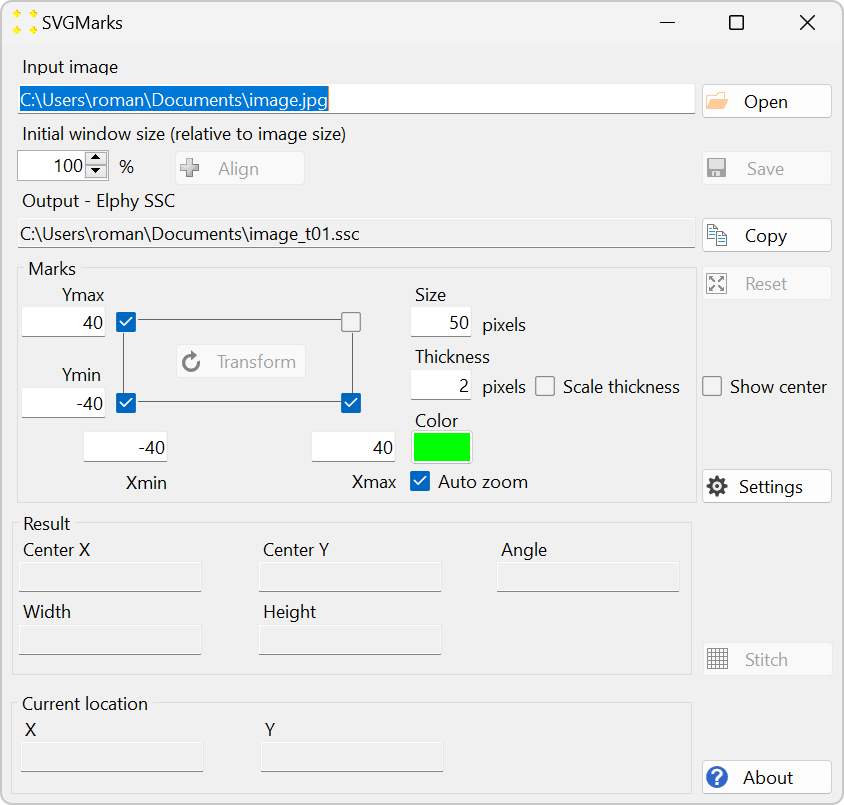
Figure 2. The main window of SVGMarks. The text box at the top ("Input image") contains the file name of the image to be processed. Initially, the program offers image.jpg stored in your personal folder (as an example - this image probably does not exist on your PC). The text box "Output - Elphy SSC" contains the name of the output SSC file, which will be created by SVGMarks during processing in the same folder (its name is derived from the file name of the input image).
Click the "Open" button to open the image you want to transform. If you prefer, you can type the full file name in the text box instead of browsing for the image. If you choose to type, press the Enter key when you are finished to tell the program that your input is finished and that you want to open the image. The selected image will instantly open in a separate window, as shown in Figure 3.
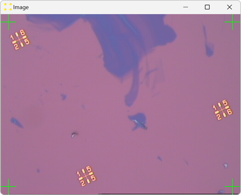
Figure 3. Opened optical image with transformation marks (green marks are used in this example; the color can be changed, as discussed below) placed by SVGMarks. The image shows graphene flakes of different thicknesses (from a monolayer to a thick multilayer). Three gold marks (in yellow), patterned by electron-beam lithography, are also visible. They define the local coordinate system of the image. In this image, the sample is deliberately rotated counter-clockwise by about 26 degrees to demonstrate the capabilities of SVGMarks. In reality, the axes of the local coordinate system should be as parallel as possible to the edges of the image (i.e., the line connecting the two lowest patterned marks should be as parallel as possible to the horizontal edge of the image).
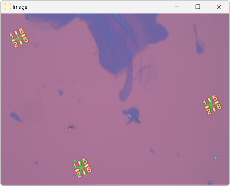
Use the mouse to place the green marks roughly over the corresponding gold marks in the image, as shown in Figure 4. To move the green mark, click anywhere within the square that defines the green mark, then drag the green mark to the desired location. The best image correction is achieved with three green marks, in which case SVGMarks applies both rotation and shear transformations to the image. The unused fourth green mark is ignored (the check boxes are used to tell the program which marks to use, as discussed below). If there are only two patterned gold marks in the image, please use only two corresponding green marks (in this case SVGMarks will only rotate the image). SVGMarks does not currently support image transformation using all four marks (i.e., one mark is always ignored).
Figure 4. Three green marks are placed over the gold marks in the image.
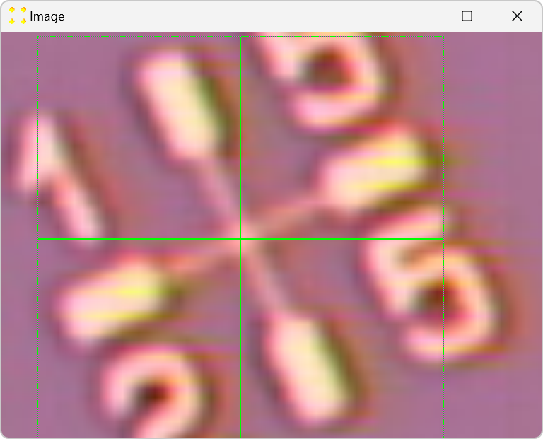
To fine-tune the position of a green mark, double-click anywhere within the square that defines the green mark. This will zoom in on the green mark, as shown in Figure 5. Alternatively, click once on the green mark to select it and then press key 3 (or 4) to zoom in on the mark (this shortcut is implemented for users of the previous version SVGMarks 3.x, which used Inkscape for mark positioning). In the zoomed image, use the mouse again to fine tune the green mark so that its center coincides with the center of the patterned gold mark. When the fine adjustment is complete, double-click inside the green mark again to zoom out. Alternatively, click once on the green mark to select it and then press key 3 (or 4) to zoom out. This procedure should be repeated for all marks.
Figure 5. The selected green mark (the one in the bottom left corner) is zoomed in and placed over the gold mark in the image.
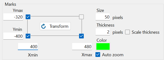
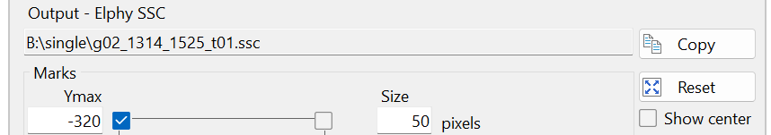
Use the check boxes shown in Figure 6 to select which green marks should be used to transform the image. In the previous example, three marks were used (in the bottom left, bottom right, and top left corner) and their check boxes should be checked. Type the coordinates of the marks in the corresponding text boxes "Xmin", "Xmax", "Ymin", and "Ymax" next to the check boxes. Values and units should correspond to the design file. In this case, the coordinates are x = 400 µm, y = -400 µm (mark in the bottom left corner), x = 480 µm (mark in the bottom right corner), and y = -320 µm (mark in the top left corner).
Figure 6. The selection of check boxes and coordinates that correspond to this example.
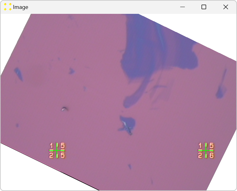
Click the "Transform" button shown in Figure 6. The transformed image is immediately displayed in the image window shown in Figure 7.
Figure 7. After the transformation, the transformed image is displayed in the same image window in which the original image was opened (see Figure 3).
The transformed image is saved in BMP format (the file name is in the text box “Output - Transformed BMP image”) in the folder of the original file, as shown in Figure 2 and Figure 8. Besides the transformed image, the program also creates two auxiliary SVG files and one SSC file. The latter file is used to place the transformed image in the design file opened in Raith Nanosuite.
Figure 8. All files are saved in the same folder as the original image. In addition to the input image and the output SSC file, SVGMarks also creates the transformed image in BMP format (this image will be displayed in the design file) and two auxiliary files in SVG format.
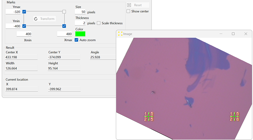
The coordinates of the image center and the image dimensions are displayed in the Result group at the bottom of the main SVGMarks window, as shown in Figure 9. These data can be used to correctly place the image in the design file other than Raith Nanosuite. After the transformation, the program knows the coordinate system of the transformed image. Consequently, hovering the mouse over the transformed image will display the mouse coordinates in the Current location group at the bottom of the main SVGMarks window.
Figure 9. The "Result" group shows the coordinates of the center of the transformed image, the angle by which the original image was rotated (provided only as a reference because the transformed image will be used in the design), and the width and height of the transformed image. The "Current location" group shows the coordinates of the mouse when it hovers over the transformed image. In this example, the mouse hovers over the mark in the bottom left corner.
The transformed image is ready to be imported into the design file because both files have the same coordinate systems. The following part of the manual explains how to place the transformed image into the Raith Nanosuite design file (keep SVGMarks open).
Click the "Copy" button to copy the file name of the SSC file, see Figure 10. SVGMarks can now be closed if it is not needed.
Figure 10. The "Copy" button is used to copy the file name of the SSC file to the Windows clipboard.
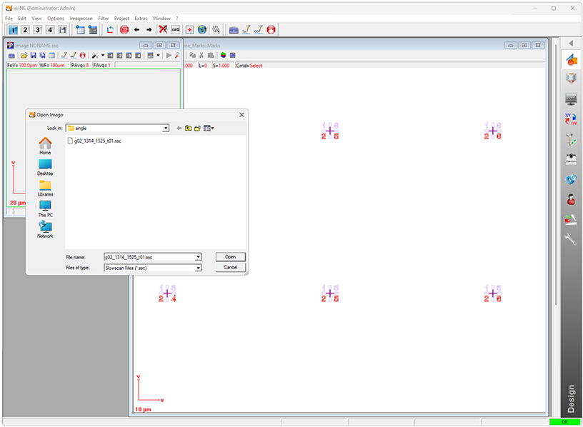
Open the design file in Raith Nanosuite. The design file corresponding to the image in this example is shown in Figure 11. To open the transformed image, click on "File" → "Open image..." and paste the file name you copied above (see Figure 10) into the "File name" text box of the "Open Image" dialog. Click "Open" to open the transformed image.
Figure 11. Raith Nanosuite with the open design file (large white window on the right). To open the transformed image, paste the SSC file name into the "File name" text box of the "Open Image" dialog.
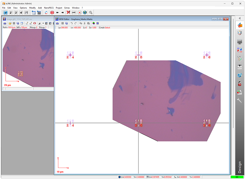
To show the transformed image in the design file, click on the design file window to bring it to the foreground, and then click "Options" → "Show Video. The transformed image will appear in the design file, as shown in Figure 12.
Figure 12. Transformed image placed at its position in the design file.
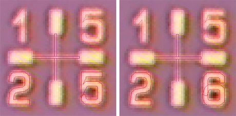
The fine alignment of the transformed image can be seen by zooming in on the visible marks, as shown in Figure 13.
Figure 13. Enlarged portions of the design file around marks showing the fine alignment of the transformed image with respect to the design file.
Design your pattern...
Stitching
SVGMarks can automatically transform multiple images based on the transformation of a given image. This is useful in situations where multiple images are taken by a microscope with a motorized stage, which introduces the same distortion in all the images. SVGMarks can be used to transform all the images at once, based on the previous transformation of one of the images.
This process is called "stitching" because it also allows all the transformed images to be stitched together into a single large image. Such image stitching is also useful when the microscope cannot take the large image at the same (high) resolution as the small images.
The images can be stitched together in two ways:
Transforming each of the small images and then stitching them together into one large image in the design file. This is the approach used by SVGMarks, as described in the example below.
Stitching the small images together and transforming only the large image. This approach does not require a design file to access the stitched image (i.e., the stitched image can be opened in any image viewer/editor) and will be available in the next version of SVGMarks.
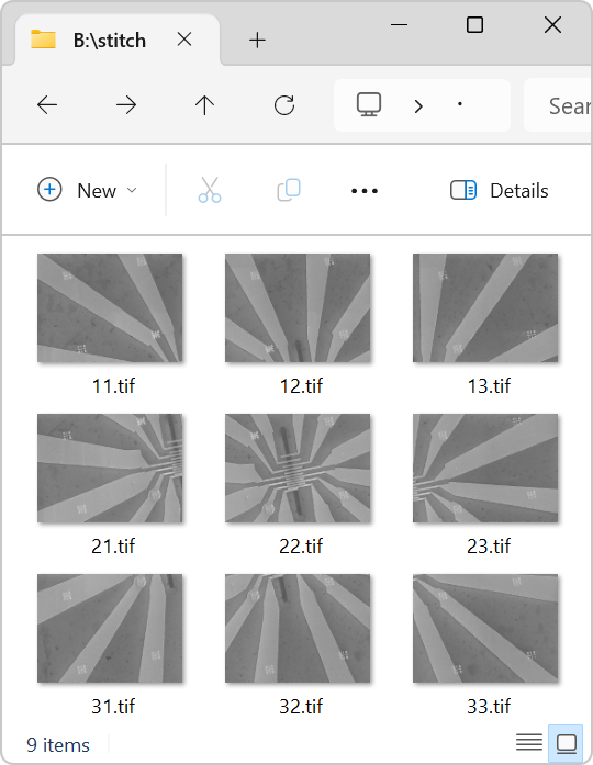
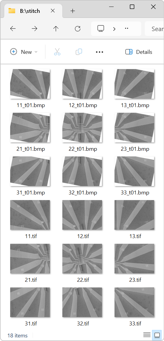
Figure 14 shows the content of a folder containing 9 images taken with a scanning electron microscope (SEM). The images are intentionally rotated about 11 degrees counterclockwise to demonstrate the capabilities of SVGMarks.
Figure 14. Images taken by an SEM with a motorized stage with a pitch of 80 µm along the axes of the local coordinate system (see Figure 18 for more details). The large image of the sample can be obtained by stitching the images in a 3 by 3 matrix.
To stitch the distorted images together, first, one of the images is transformed using SVGMarks as explained in Processing a single image. Second, the same transformation is applied to all images. Third, the transformed images are stitched together. The whole procedure is explained below.
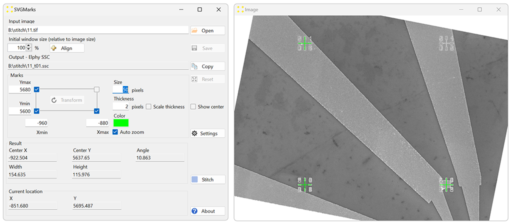
Transform one of the images with SVGMarks as explained in Processing a single image. The choice of the image is arbitrary, but to simplify the stitching procedure, it is recommended to transform the image which is physically located in one of the corners of the structure. In the example shown in Figure 14, the image "11.tif" is selected. Figure 15 shows the result of transforming image "11.tif".
Figure 15. The result of the transformation of the image "11.tif".
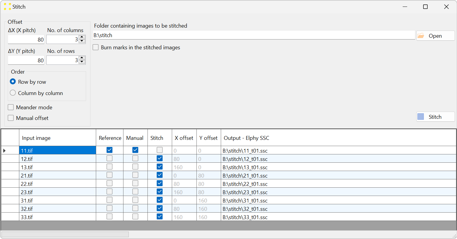
Click the "Stitch" button to open the "Stitch" window shown in Figure 16.
Figure 16. The "Stitch" window, where you can define the images to be transformed and the corresponding stitching parameters.
the image transformed in the previous step ("11.tif") is the reference image with respect to which all other images should be transformed;
all images to be transformed are located in the same folder as the reference image.
In the table at the bottom of the window, SVGMarks lists all images found in the folder of the reference image. If the images to be transformed are located in a different folder, click the "Open" button to browse for one of the images you want to transform. Once the image is selected, its folder will be used.
The table has the following columns:
The "Input image" column contains the names of the reference image and the images to be transformed using the same transformation previously applied to the reference image.
The "Reference" column contains check boxes indicating which image is the reference image. By default, SVGMarks always selects the previously transformed image (in this case "11.rtf") as the reference image. However, users have the option to choose the reference image by checking the corresponding check box in the "Reference" column. The reference image will not be transformed as SVGMarks assumes that the reference image has already been transformed.
The "Manual" column is a read-only column that indicates the images that have already been transformed by SVGMarks. This is to inform users that the images, whose check boxes are checked, have already been transformed by SVGMarks and that they may not require the automatic transformation by the "Stitch" option.
The "Stitch" column indicates which images should be transformed. By default, SVGMarks selects all images apart from the reference image to be transformed. Users have the option to exclude some of the images from the transformation by unchecking their check boxes.
The columns "X offset" and "Y offset" contain image offsets along the x and y axes, respectively. SVGMarks will not only transform the images selected in the column "Stitch", but also translate them by the corresponding "X offset" and "Y offset" along the x and y axes, respectively. These offsets are calculated with respect to the reference image (hence zero offsets of the reference image) based on the entries in the group "Offset", as discussed further below. However, if the check box "Manual" is checked, the values in these two columns can be edited manually.
The column "Output - Elphy SSC" contains the full file names of the SSC files that will be generated by transforming the images.
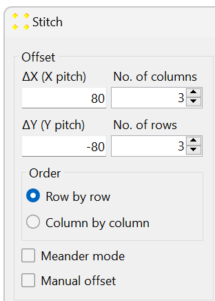
The group "Offset", shown in Figure 16 and Figure 17, is used to automatically calculate the offset of the images to be transformed with respect to the reference image. In the case the stitching is not important, i.e, when the images should only be transformed without any translation, the group "Offset" can be disregarded.
Figure 17. The "Offset" group contains settings that are used to translate the images with respect to the reference image.
The images are listed in alphabetical order in the table. The radio buttons in the subgroup "Order" are used to select the order in which they are placed in the actual structure. This is demonstrated by Figure 18. The first three images in the table (11.rtf, 12.rtf, and 13.rtf) form the top row of the structure. The next three images (21.rtf, 22.rtf, and 23.rtf) form the middle row of the structure. The final three images (31.rtf, 32.rtf, and 33.rtf) form the bottom row of the structure. The images are therefore ordered in a row-by-row format in the table, which means that users should check the "Row by row" check box.
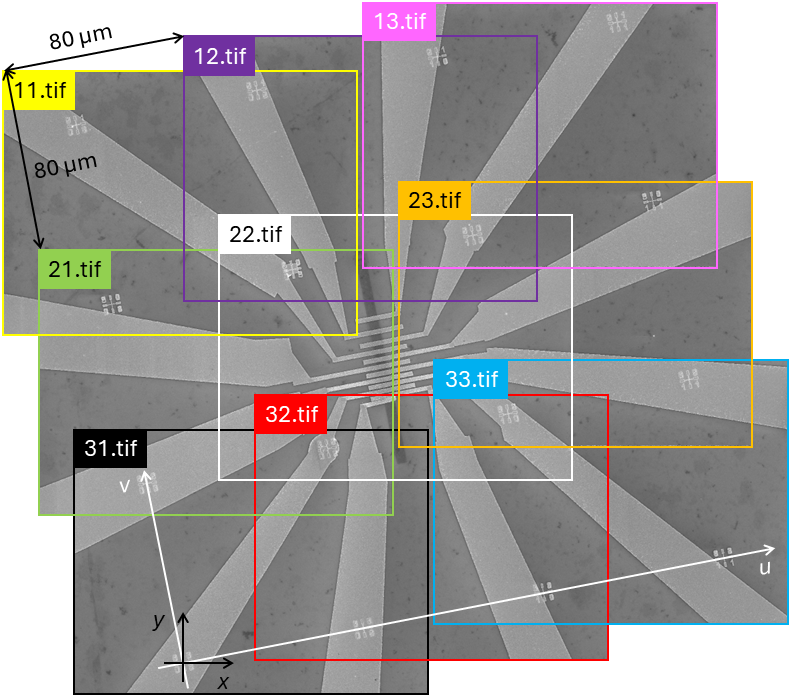
Figure 18. The image of the structure was obtained by manually stitching the images shown in Figure 14. The sample was mounted in an SEM with a large rotation of about 11 degrees counter-clockwise to demonstrate the capabilities of SVGMarks. In reality, the rotation should be minimized, but zero rotation is not possible, even with great care. The coordinate system has been aligned with respect to the alignment marks (the local Cartesian coordinate system of the sample is denoted by u-v). The images are taken by moving the laser stage with a pitch of 80 µm along both the u and v axes. If all the images are transformed so that the u-v system becomes identical to the x-y system, then a pitch of 80 µm can be used along both the horizontal (x) and vertical (y) axes to stitch the images together.
Given that the reference image is located in the top left corner, the offsets along the x and y axes are 80 µm and -80 µm, respectively. Consequently, "ΔX (X pitch)" and "ΔY (Y pitch)" should be set to 80 and -80 in Figure 17, respectively. Finally, the images are arranged in a 3 by 3 matrix. Therefore, both the "No. of columns" and "No. of rows" should be set to 3 in the group "Offset" shown in Figure 17.
The "Meander" check box should be selected if the images are ordered in a meander fashion in the table, which is not the case here. In that case, the meander order would be 11.tif, 12.tif, 13.tif, 23.tif, 22.tif, 21.tif, 31.tif, 32.tif, and 33.tif.
To perform both transformation and stitching (translation) of the selected images, click the "Stitch" button. In this example, SVGMarks will generate bitmap (BMP), SVG, and SSC images for each of the images in the folder (apart from the reference image 11.tif) as if they were manually transformed. The image content of the folder is shown in Figure 19. The first nine images displayed in the figure are transformed bitmap images.
Figure 19. Part of the folder content after stitching. Only images are shown.
Open the design file in Raith Nanosuite. To open the transformed images, click on "File" → "Open image..." and choose one of the images, e.g., 11.rtf. Repeat until all images are open.
To show the transformed images in the design file, click on the design file window to bring it to the foreground, and then click "Options" → "Show Video. The transformed images will appear in the design file, as shown in Figure 20.
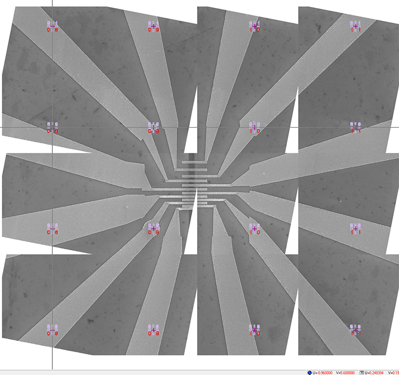
Figure 20. The stitched transformed SEM images in the design file. The white triangles within the image are a consequence of a significant (deliberate) rotation of the individual images. It is recommended that the images be taken with the smallest possible rotation.
Other controls and actions
The following list explains the controls and actions in the main SVGMarks window that were not used in the above manual.
If you are not satisfied with the transformation, you can return to the original (untransformed) image by clicking the 'Align' button.
When you click the "Transform button", the position of the marks in the original (untransformed) image is automatically saved before the transformation is performed and the transformed image is opened. If you want to save the position of the marks in the untransformed image for a later session (without transforming the image), click the "Save" button.
If you want to open an image that has previously been transformed, click the "Open" button and open the original (untransformed) image. Once the image is open, SVGMarks will set the mark location in the image (Figure 4) and the transformation parameters (Figure 6) as they were set the last time the image was transformed. If you would like to see the transformed image, click the button "Transform".
By default, SVGMarks opens images in their original resolution. This can be a problem if, for example, the image was taken at a higher resolution than that of the screen. In this case, the image window will be larger than the desktop. Although a user can resize the image window, it is more convenient to tell SVGMarks to open the resized image window from the start. Use the numeric field "Initial window size (relative to image size)" to set the ratio between the resolution of the image window and the image. For example, if this numeric field is set to 50 % before opening an image, the displayed image will have half the resolution of the original image (it will be twice as small as the original image).
The position of the marks in the image window can be reset by clicking the "Reset" button.
To manually zoom in/out, scroll the mouse wheel. In this case, the image is zoomed in/out relative to the center of the image window. Double-click on any feature in the image to move it to the center of the image window. If the feature is within the square defined by a mark, uncheck the "Auto zoom" check box to avoid zooming in/out on the mark.
If you double-click outside the square defined by a mark during mark positioning (Figure 4 and Figure 5), the image will be centered at the point where you double-clicked (i.e., the image will be moved within the image window instead of zoomed to a mark). The position of the image within the image window has no effect on the image transformation. However, if you prefer to return the image in the center of the image window, you can:
double-click on the mark (to zoom in) and then double-click again to zoom out (this is the quickest way to re-center the image as the images are always centered when you zoom out) or
double-click on the actual center of the image (which is not always easy to find) or
click the "Reset" button (this will also reset the position of the marks, which is the main purpose of this button).
The numeric fields "Size" and "Thickness" set the dimensions of the marks in the image window (in pixels). The "Color" button sets the color of the marks in the image window. Changing any of these settings will immediately change the appearance of the marks in the image window.
When an image is opened for the first time, the thickness of the marks is set using the 'Thickness' numeric field. In the example above, the mark thickness was set to 2 pixels. Double-clicking on a mark will zoom the image to the mark by an appropriate factor (Figure 5). If the 'Scale thickness' check box is unchecked, as in the example above, the thickness of the zoomed mark will not change (it will remain 2 pixels in the example above). However, if this check box is checked, the thickness of the zoomed mark will be increased by the same zoom factor.
Check the "Show center" check box to display the center of the image window.